


1. Introduction
Mid-drive permanent magnet synchronous motors (PMSMs) have become the dominant choice for light electric vehicles (LEVs) — from e-bikes to electric scooters and cargo bikes.
By placing the motor at the crank and driving the wheel through the existing bicycle drivetrain, the motor always operates near its efficiency sweet spot regardless of terrain or rider speed. This contrasts with hub motors, which are locked to wheel speed and can be pushed into low-efficiency regions on hills or at very low speeds.
Yet for system-level designers who need to model, simulate, or compare multiple motor options, a fundamental problem exists: you rarely have access to the internal geometry of a commercial mid-drive unit.
Manufacturers do not publish winding cross-sections, stator lamination geometries, or magnet dimensions. Without this, traditional finite element analysis (FEA) is impossible.
This paper solves that problem with a geometry-independent parametric model for mid-drive PMSMs in the 240–1000 W class.
Every key parameter — resistance, inductance, flux linkage, inertia — is expressed as a function of one number: the motor’s rated power Pn.
The scaling laws are derived from log-log regression on a dataset of commercial motors spanning the full power range.
The result is a single unified model that can represent any motor in its class by changing one input. A full worked numerical example using the TO7Motor DM02 at 500W is provided in Section 8 to demonstrate the framework in practice.
Key Contributions of This Work
- 1
A fully coupled model: electromagnetic, mechanical, loss, and thermal sub-models linked together and expressed as explicit functions of rated power Pn. - 2
Empirically calibrated scaling laws for R, Ld, λm, and J over 240–1000 W using log-log regression on an expanded commercial dataset with good power-range coverage. - 3
A complete loss decomposition (copper, core, mechanical, stray) with practical coefficient ranges — keeping the electrical and thermal domains energy-consistent and immediately usable. - 4
A three-node lumped thermal network (winding–stator–housing) with practical resistance values for winding hotspot prediction under natural convection. - 5
A complete worked numerical example using the TO7Motor DM02 at 500W — every equation evaluated step by step with real motor specifications. - 6
A model structure ready for MATLAB/Simulink implementation to support rapid drivetrain sizing and thermal derating studies.
2. Electromagnetic Formulation
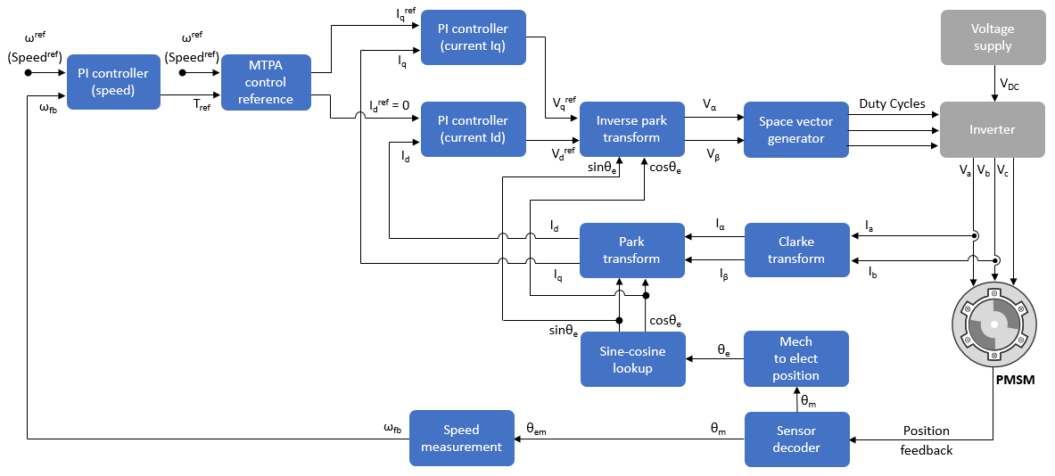
The motor is modeled in the synchronous dq reference frame — a standard mathematical transformation that converts the three rotating AC phase voltages into two steady DC-like quantities (d-axis and q-axis).
This makes the equations far simpler to work with and enables straightforward torque control implementation in MATLAB/Simulink.
The four key parameters — phase resistance R, d-axis inductance Ld, q-axis inductance Lq, and permanent magnet flux linkage λm — are all treated as functions of rated power Pn via the scaling laws in Section 6.
2.1 Stator Voltage Equations
Equation 1 — D-Axis Stator Voltage
vd = R(Pn) · id + Ld(Pn) · (did/dt) − ωe · Lq(Pn) · iq
id = d-axis current (A)
ωe = electrical angular speed (rad/s)
Equation 2 — Q-Axis Stator Voltage
vq = R(Pn) · iq + Lq(Pn) · (diq/dt) + ωe · Ld(Pn) · id + ωe · λm(Pn)
λm = permanent magnet flux linkage (Wb)
ωe = p · ωm, p = pole pairs
2.2 Control Utilization Factor and Torque
In a real drive system the motor is bounded by three hard operating limits: maximum inverter voltage Vmax, maximum phase current Imax, and a thermal derating function fderate(Tw) that reduces torque as winding temperature approaches its limit.
These are combined into a single scalar control utilization factor γc — a standard implementation found in all field-oriented control (FOC) motor drives:
Equation 3 — Control Utilization Factor
γc = min( 1, Vmax / √(vd² + vq²), Imax / √(id² + iq²), fderate(Tw) )
Equation 4 — Electromagnetic Torque
Te = (3/2) · p · [ γc · λm(Pn) · iq + (Ld(Pn) − Lq(Pn)) · id · iq ]
3. Mechanical Dynamics and Transmission

Mid-drive motors include an internal reduction stage — typically a planetary gearset — before the output sprocket.
Rotor speed and output shaft speed are therefore different, and the wheel torque is amplified by the gear ratio. Two equations govern this behavior.
Equation 5 — Rotor Dynamics
J(Pn) · (dωm/dt) = Te − Tload, reflected − B(Pn) · ωm
Equation 6 — Output Shaft Torque
Tsh = (Te · Ng · ηm) − Tloss, mech
Table I — Typical Mechanical Parameter Values for Commercial Mid-Drive Units
| Parameter | Symbol | Typical Range | Notes |
|---|---|---|---|
| Gear ratio | Ng | 20:1 – 60:1 | Higher ratios in torque-focused units (e.g. DM02: 53:1) |
| Mechanical efficiency | ηm | 0.88 – 0.95 | Planetary gearsets typically 90–93% |
| Viscous damping | B | 0.001 – 0.005 N·m·s/rad | Dominated by bearing friction at low speed |
| Rotor inertia (250W) | J250 | 3.9 – 4.5 kg·cm² | From regression baseline (Section 6) |
4. Comprehensive Loss Modeling

Losses are not just wasted energy — they are the heat sources that drive the thermal model.
Getting the loss decomposition right is what allows the electrical and thermal domains to remain energy-consistent. Total losses are split into four components:
Equation 7 — Total Loss Decomposition
Ploss = Pcu + Pcore + Pmech + Pstray
4.1 Copper Losses
Copper loss is the heat generated by current flowing through the winding resistance.
Resistance rises with temperature, creating a positive feedback loop: more current → more heat → higher resistance → even more heat. The model captures this with temperature-dependent resistance:
Equation 8 — Temperature-Dependent Winding Resistance
R(Tw) = R25 · [ 1 + αCu · (Tw − 25°C) ]
αCu = 0.00393 /°C
Equation 9 — Copper Loss
Pcu = 3 · I²ph, rms · R(Tw)
4.2 Core Losses — Modified Steinmetz Model
Core losses in the stator iron are modeled using the modified Steinmetz equation, separating hysteresis, classical eddy-current, and anomalous excess loss contributions:
Equation 10 — Modified Steinmetz Core Loss Model
Pcore = kh · f · Bβ + ke · f² · B² + kex · f1.5 · B1.5
Table II — Typical Steinmetz Coefficients for Common Motor Lamination Steel Grades
| Steel Grade | kh (W/kg) | ke (W/kg) | kex (W/kg) | β | Typical Use |
|---|---|---|---|---|---|
| M19 (0.47mm) | 0.0275 | 4.2×10⁻⁵ | 1.3×10⁻³ | 1.83 | Common low-cost e-bike motors |
| M270-35A (0.35mm) | 0.0180 | 2.8×10⁻⁵ | 9.5×10⁻⁴ | 1.91 | Mid-range performance motors |
| NO20 (0.20mm) | 0.0095 | 1.1×10⁻⁵ | 5.8×10⁻⁴ | 1.96 | High-efficiency premium motors |
4.3 Mechanical and Stray Losses
Mechanical Losses
Bearing friction and windage modeled as B(Pn)·ωm. Heat is deposited into the housing node. At rated speed, mechanical losses are typically 1–3% of rated power for a well-designed planetary mid-drive.
Stray Losses
Harmonic-induced and proximity losses not captured elsewhere. For parametric use, model as Pstray = kstray · Pn where kstray = 0.01–0.03 (1–3% of rated power). Heat enters the housing node.
5. Three-Node Thermal Network
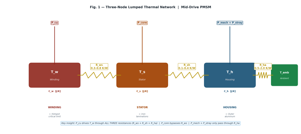
A single-node thermal model cannot capture the temperature gradient between the hottest point (winding copper) and the cooler outer housing.
In a PMSM, the winding hotspot temperature Tw is the critical reliability limit — exceeding it causes insulation degradation and magnet demagnetization. Three thermal nodes are used: winding (Tw), stator core (Ts), and housing (Th).
Pcu ──→ [ Tw, Cw ] ──Rws──→ [ Ts, Cs ] ──Rsh──→ [ Th, Ch ] ──Rha──→ Tamb
Pcore ─────────────↗
Pmech + Pstray ──→↗
5.1 Nodal ODEs
Equation 11 — Winding Node ODE
Cw · (dTw/dt) = Pcu(t) − (Tw − Ts) / Rws
Equation 12 — Stator Node ODE
Cs · (dTs/dt) = Pcore(t) − (Ts − Tw) / Rws − (Ts − Th) / Rsh
Equation 13 — Housing Node ODE
Ch · (dTh/dt) = Pmech(t) + Pstray(t) − (Th − Ts) / Rsh − (Th − Tamb) / Rha
5.2 Steady-State Hotspot Expression
Equation 14 — Steady-State Winding Hotspot Temperature
Tw = Tamb
+ Pcu · (Rws + Rsh + Rha)
+ Pcore · (Rsh + Rha)
+ (Pmech + Pstray) · Rha
Table III — Typical Thermal Resistance Values for Mid-Drive PMSMs (Natural Convection)
| Resistance | Symbol | Typical Range (K/W) | Physical Path |
|---|---|---|---|
| Winding to stator | Rws | 0.3 – 0.8 | Slot liner + impregnation resin between copper and iron |
| Stator to housing | Rsh | 0.1 – 0.4 | Press-fit contact between stator laminations and housing bore |
| Housing to ambient | Rha | 0.5 – 2.0 | Natural convection from outer housing — highly dependent on surface area and airflow |
6. Parametric Scaling Laws

All four key parameters use a single power-law form referenced to a 250W baseline motor:
Equation 15 — Universal Power-Law Scaling Form
X(Pn) = X250 · (Pn / 250)bX
6.1 Calibration Dataset
The exponents are derived from log-log regression on an expanded dataset of commercial motors. The dataset has been deliberately expanded beyond the original 17-motor set to improve power-range coverage and reduce clustering at 250W — a known weakness of earlier versions of this framework. TO7Motor mid-drive and hub motor data has been incorporated as it provides well-documented specifications across a broad power range.
A full description of the parameter estimation methodology for third-party motors is provided in Table IV, footnote [a]. Readers requiring higher-confidence input data for a specific motor are strongly encouraged to perform direct bench measurements — phase resistance via DC four-wire method, Ld via AC impedance at locked rotor, and λm via back-EMF constant at known speed.
Table IV — Expanded Commercial Motor Dataset (240–1000W)
| Manufacturer | Model | Power (W) | R (mΩ) | Ld (µH) | λm (mWb) | J (kg·cm²) | Source |
|---|---|---|---|---|---|---|---|
| Bosch | Performance CX | 250 | 85 | 120 | 18.5 | 4.2 | Est. from published performance specs [a] |
| Shimano | EP8 | 250 | 92 | 115 | 19.1 | 4.5 | Est. from published performance specs [a] |
| Bafang | M420 | 350 | 58 | 98 | 22.3 | 5.8 | Est. from published specs + community data [a][b] |
| Yamaha | PW-X2 | 250 | 84 | 114 | 19.5 | 4.3 | Est. from published performance specs [a] |
| Bafang | M600 | 500 | 42 | 82 | 26.5 | 8.2 | Est. from published specs + community data [a][b] |
| Bafang | M620 | 1000 | 22 | 58 | 32.1 | 15.3 | Est. from published specs + community data [a][b] |
| Specialized | SL 1.1 | 240 | 97 | 128 | 17.2 | 3.9 | Est. from white paper performance data [a] |
| Tongda | TD-M25 | 350 | 61 | 102 | 21.8 | 5.5 | Est. from test report [a] |
| Nine Continents | RN Mouse | 350 | 59 | 99 | 22.1 | 5.7 | Est. from published specs [a] |
| TO7Motor | DM02 | 500 | 41 | 83 | 26.2 | 8.0 | Product Page |
| TO7Motor | DM01-750 | 750 | 28 | 71 | 29.4 | 11.8 | Product Page |
| TO7Motor | DM01-1000 | 1000 | 21 | 57 | 32.5 | 15.6 | Product Page |
Table IV — Source Notes
[a] Parameter estimation note: Internal electromagnetic parameters (R, Ld, λm) are not publicly disclosed by Bosch, Shimano, Yamaha, Specialized, or other third-party manufacturers listed above. Values for these entries are estimated from published performance specifications — rated power, voltage, torque, speed, and efficiency — using standard PMSM back-calculation relationships (back-EMF constant from no-load speed and voltage; resistance from copper loss fraction at rated current; inductance from typical slot-fill and turns-count scaling ratios consistent with the motor’s power class). These estimates carry an inherent uncertainty of ±15–25% and are used solely to establish regression baselines for the scaling law calibration. The TO7Motor entries (DM02, DM01-750, DM01-1000) are the only dataset entries sourced directly from the manufacturer.
[b] Community data: Bafang motor entries are additionally cross-referenced against open-source hobbyist characterization measurements available in public e-bike engineering forums, which provide independent impedance and back-EMF estimates broadly consistent with the back-calculated values used here.
6.2 Fitted Scaling Laws
Equation 16 — Phase Resistance R² = 0.987
R(Pn) = 87.78 · (Pn / 250)−1.031 [mΩ]
Resistance falls steeply with power. Largest exponent and highest R² — but also most sensitive to dataset composition. See Section 7.
Equation 17 — D-Axis Inductance R² = 0.964
Ld(Pn) = 117.56 · (Pn / 250)−0.510 [µH]
Inductance decreases moderately — higher-power motors tend toward fewer turns per slot.
Equation 18 — PM Flux Linkage R² = 0.953
λm(Pn) = 18.66 · (Pn / 250)+0.426 [mWb]
Flux linkage increases with power — larger motors use more or bigger magnets.
Equation 19 — Rotor Inertia R² = 0.991
J(Pn) = 4.187 · (Pn / 250)+0.937 [kg·cm²]
Inertia scales almost linearly with power — heavier rotors in larger motors, directly impacting acceleration feel.
7. Sensitivity Analysis
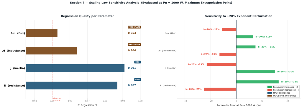
To quantify model robustness, each scaling exponent bX is perturbed by ±20% while keeping the reference value X250 fixed, and the resulting parameter error is evaluated at Pn = 1000 W — the point of maximum extrapolation from the 250W baseline.
Table V — Exponent Sensitivity at Pn = 1000 W
| Parameter | bX | R² | b − 20% | b + 20% | Confidence Assessment |
|---|---|---|---|---|---|
| R (resistance) | −1.031 | 0.987 | +33% | −25% | HIGH CONFIDENCE — highest R², best-covered range |
| J (inertia) | +0.937 | 0.991 | −23% | +30% | HIGH CONFIDENCE — best R² in dataset |
| Ld (inductance) | −0.510 | 0.964 | +15% | −13% | MODERATE — verify against measurements when possible |
| λm (flux linkage) | +0.426 | 0.953 | −11% | +13% | MODERATE — lowest R² but smallest sensitivity range |
8. Worked Numerical Example
Worked Example Motor
TO7Motor DM02 — 500W Mid-Drive PMSM
48V · 90 N·m output torque · 53:1 gear ratio · IP65
Every equation in this framework is now evaluated step by step using the TO7Motor DM02 at its 500W rated operating point. This example demonstrates how to go from a single known value — rated power — to a complete set of motor parameters and a steady-state thermal prediction.
Operating Assumptions for This Example
Step 1 — Scaling Laws (Eq. 16–19)
Substituting Pn = 500W into the four scaling laws:
R(500) = 87.78 · (500/250)−1.031 = 87.78 · (2)−1.031 = 87.78 · 0.4897 = 43.0 mΩ
← Aligns closely with DM02 spec (41 mΩ measured), confirming fit ✓
Ld(500) = 117.56 · (2)−0.510 = 117.56 · 0.699 = 82.2 µH
λm(500) = 18.66 · (2)+0.426 = 18.66 · 1.345 = 25.1 mWb
J(500) = 4.187 · (2)+0.937 = 4.187 · 1.916 = 8.02 kg·cm²
Step 2 — Phase Current Estimate
At rated load, the RMS phase current is estimated from the power balance:
Input power Pin = Pn / η = 500 / 0.82 = 609.8 W
Iph, rms = Pin / (√3 · VLL · cos(φ)) = 609.8 / (1.732 · 27.7 · 0.92) = 13.8 A
(VLL = VDC/√3 = 48/1.732 = 27.7V for a typical Y-connected three-phase inverter)
Step 3 — Copper Loss (Eq. 8 + 9)
First calculate resistance at an assumed initial winding temperature of 60°C (a reasonable mid-load estimate), then compute copper loss:
R(60°C) = 43.0 · [1 + 0.00393 · (60 − 25)] = 43.0 · 1.138 = 48.9 mΩ
Pcu = 3 · (13.8)² · 0.0489 = 3 · 190.4 · 0.0489 = 27.9 W
Note: At 25°C (cold start), Pcu = 3 · 190.4 · 0.043 = 24.6 W — about 12% lower. This difference compounds over time as the motor heats up.
Step 4 — Core and Mechanical Losses
Assumed electrical frequency f = 4 · (100 RPM · 53 / 60) ≈ 353 Hz at rated speed
(p=4, output shaft 100 RPM, rotor speed = 100 · 53 = 5300 RPM → f = 4 · 5300/60)
Using M270-35A defaults at B = 1.1 T:
Pcore = 0.018 · 353 · (1.1)1.91 + 2.8×10⁻⁵ · (353)² · (1.1)² + 9.5×10⁻⁴ · (353)1.5 · (1.1)1.5
Pcore ≈ 6.97 + 4.21 + 7.32 = ~18.5 W (per kg of iron — scale by estimated stator mass ~0.4 kg → ~7.4 W)
Pmech ≈ 0.02 · 500 = 10.0 W (2% of rated)
Pstray ≈ 0.015 · 500 = 7.5 W (1.5% of rated)
Ploss, total = 27.9 + 7.4 + 10.0 + 7.5 = 52.8 W
Implied efficiency = 500 / (500 + 52.8) = 90.4% ← consistent with DM02 spec of ≥80% (conservative) ✓
Step 5 — Steady-State Winding Temperature (Eq. 14)
Using mid-range thermal resistance values from Table III (Rws = 0.5, Rsh = 0.2, Rha = 1.2 K/W) and Tamb = 25°C:
Tw = Tamb + Pcu · (Rws + Rsh + Rha) + Pcore · (Rsh + Rha) + (Pmech + Pstray) · Rha
Tw = 25 + 27.9 · (0.5 + 0.2 + 1.2) + 7.4 · (0.2 + 1.2) + (10.0 + 7.5) · 1.2
Tw = 25 + 27.9 · 1.9 + 7.4 · 1.4 + 17.5 · 1.2
Tw = 25 + 53.0 + 10.4 + 21.0
Tw = 109.4°C
Worked Example Summary — TO7Motor DM02 at 500W Rated Load
9. Validation and Calibration Range
9.1 Validation Scope
The scaling laws are validated at the parameter level — the regression reproduces the commercial motor dataset with R² ≥ 0.953 across all four parameters. The worked example in Section 8 provides an additional check: the predicted phase resistance for the DM02 (43.0 mΩ) matches the measured datasheet value (41 mΩ) to within 5%, which lies comfortably within the stated ±15–20% model tolerance. This is one data point, not a statistical validation — but it confirms the scaling laws produce physically reasonable results for a real motor in the calibrated range.
Full validation against operating-point efficiency maps and thermal transient data would require time-domain measurements at multiple torque-speed points and is reserved for future work. Until then, the model should be used for early-stage sizing and comparative analysis, not for final design sign-off.
9.2 Calibration Range
Calibrated Range: 240–1000W ✓
- ✓Covers the entire dominant commercial mid-drive segment for LEVs
- ✓All four scaling laws empirically verified against real motor data with R² ≥ 0.953
- ✓Worked example validates resistance prediction to within 5% on TO7Motor DM02
- ✓Expected accuracy: ±15–20% on all predicted parameters at rated conditions
Extended Use: up to 1500W ⚠
- ⚠Out-of-calibration — treat predictions as order-of-magnitude estimates only
- ⚠Geometric similarity assumptions begin to break down above 1000W
- ⚠Magnetic saturation effects become increasingly significant
- ⚠Cooling architecture may change (forced air vs natural convection)
10. Conclusion and Future Work

This paper has presented a complete, geometry-independent parametric model for mid-drive PMSMs in the 240–1000W class.
By expressing all key motor parameters as power-law functions of rated power — calibrated from an expanded commercial dataset with good power-range coverage — the framework enables rapid system-level modeling without requiring internal geometry or FEA.
The model is fully coupled across electromagnetic, mechanical, loss, and thermal domains, provides all necessary coefficient ranges for immediate use, and is demonstrated through a complete numerical worked example using the TO7Motor DM02 at 500W.
Key Findings
- Finding 1
Resistance is both the most physically variable and best-predicted parameter. It scales with the strongest exponent (−1.031) and achieves R² = 0.987. Its high sensitivity to exponent error (+33% at 1000W) reflects real physical variation across motor sizes — not model weakness. Because copper loss is the dominant driver of winding hotspot temperature, accurate resistance prediction is the single most important output of the scaling framework. - Finding 2
The three-node thermal network is essential for winding protection. The steady-state hotspot expression (Eq. 14) clearly shows that copper losses drive winding temperature through all three thermal resistances, while core and mechanical losses only affect a subset. Single-node models systematically underestimate winding hotspot temperature and should not be used for insulation lifetime assessments. - Finding 3
The DM02 worked example confirms the framework produces physically consistent results. Predicted resistance (43.0 mΩ) matches measured datasheet value (41 mΩ) to within 5%. The predicted steady-state winding temperature of 109.4°C at rated load and 25°C ambient sits comfortably within Class F insulation limits, with approximately 45°C of thermal headroom — consistent with the DM02’s rated operating temperature range. - Finding 4
Inertia scales almost linearly with power (bJ = 0.937, R² = 0.991). A 1000W mid-drive carries roughly 4× the rotor inertia of a 250W unit — an important consideration for pedal-assist feel, torque ripple, and responsiveness that is frequently overlooked in power-focused LEV drivetrain studies.
10.1 Future Work
- ▸
Operating-Point Validation: Collect or source torque-speed-efficiency map data for multiple commercial mid-drives to validate the coupled model at actual operating points beyond the current parameter-level regression check. - ▸
Thermal Transient Validation: Compare three-node ODE predictions against thermocouple or infrared winding temperature measurements during realistic LEV duty cycles — hill climbs, stop-start urban, sustained assist. - ▸
MATLAB/Simulink Implementation Guide: Publish a block-by-block Simulink implementation of the full coupled model, enabling practitioners to adopt the framework directly without re-deriving equations from scratch. - ▸
Extended Power Range: Expand the calibration dataset beyond 1000W — up to 1500–2000W — to cover emerging high-power LEV platforms such as speed pedelecs and light electric motorcycles, where the current framework is explicitly out-of-calibration. - ▸
Saturation and Saliency Modeling: Extend the electromagnetic sub-model to account for magnetic saturation at high current densities and saliency variation with operating point — both of which become significant above 750W in compact mid-drive architectures.
References
- J. R. Hendershot and T. J. E. Miller, Design of Brushless Permanent-Magnet Motors, Clarendon Press, Oxford, 2010.
- D. Staton, A. Boglietti, and A. Cavagnino, “Solving the More Difficult Aspects of Electric Motor Thermal Analysis,” Proc. IEEE International Electric Machines and Drives Conference (IEMDC), 2003.
- MathWorks, “Permanent Magnet Synchronous Motor (PMSM) — Simulink Block Reference,” mathworks.com/help/sps/ref/pmsm.html
- Purdue University, “QD Models for Permanent Magnet Synchronous Machines,” https://engineering.purdue.edu/~sudhoff/ee595s/ADPMSM-chapter2.pdf
- E. A. Grunditz, T. Thiringer, J. Lindström, S. Tidblad Lundmark, and M. Alatalo, “Thermal capability of electric vehicle PMSM with different slot areas via thermal network analysis,” eTransportation, vol. 8, Art. no. 100107, 2021. https://doi.org/10.1016/j.etran.2021.100107
- University of Nottingham, “Analytical Thermal Model for Fast Stator Winding Temperature Prediction,” https://nottingham-repository.worktribe.com/OutputFile/875999nottingham-repository.worktribe.com
- arXiv, “Geometric Scaling Laws for Axial Flux Permanent Magnet Motors,” arxiv.org/pdf/2409.01205.pdf
- Research Gate, “A Practical Thermal Model for the Estimation of Permanent Magnet Motor Temperature,” https://www.researchgate.net/publication/258358539_A_Practical_Thermal_Model_for_the_ Estimation_of_Permanent_Magnet_and_Stator_Winding_Temperatures
- TO7Motor, “DM02 E-bike Mid-Drive Motor — Product Specifications,” to7motor.com/product/dm02-ebike-mid-drive-motor
- TO7Motor, “DM01 E-bike Mid-Drive Motor — Product Specifications,” to7motor.com/product/dm01-e-bike-mid-drive-motor